Training Parameters Tab and Settings
The Training Parameters tab, shown below, includes a set of basic settings for training a deep model, as well advanced settings that let you modify the default settings of the selected optimization algorithm and to add metric and callback functions.
Training Parameters tab

A. Basic settings B. Advanced settings
The basic settings that you need to set to train a deep model are available in the top section of the Training Parameters tab, as shown below.
Basic settings

| Description | |
|---|---|
| Input (Patch) Size |
During training, training data is split into smaller 2D data patches, which is defined by the 'Input (Patch) Size' parameter.
For example, if you choose an Input (Patch) Size of 64, the Deep Learning Tool will cut the dataset into sub-sections of 64x64 pixels. These subsections will then be used as the training dataset. By subdividing images, each pass or 'epoch' should be faster and use less memory. |
| Stride to Input Ratio |
The 'Stride to Input Ratio' specifies the overlap between adjacent patches.
At a value of '1.0', there will be no overlap between patches and they will be extracted sequentially one after another. At a value of '0.5', there will be a 50% overlap. You should note that any value greater than '1.0' will result in gaps between data patches. |
| Epochs Number | A single pass over all the data patches is called epoch, and the number of epochs is controlled by the 'Epochs Number' parameter. |
| Batch Size | Patches are randomly processed in batches and the 'Batch Size' parameter determines the number of patches in a batch. |
| Loss Function |
Loss functions, which are selectable in the drop-down menu, measure the error between the neural network's prediction and reality. The error is then used to update the model parameters.
You should note that not all the loss functions will work well with all models and the available selections are automatically filtered according to the model type — Regression (for super-resolution and denoising) and Semantic Segmentation (for binary and multi-class segmentations). Regressive loss functions… Are used in cases of regressive problems, that is when the target variable is continuous. One of the most widely used regressive loss functions is Mean Squared Error. Other loss functions you might consider are Cosine Similarity, Huber, Mean Absolute Error, Poisson, and others listed in the drop-down menu (see Loss Functions for Regression Models). Semantic segmentation loss functions… Are used in cases of segmentation problems, that is when the target output is a multi-ROI. When training a multi-class segmentation model, 'CategoricalCrossentropy' is generally a good choice as a classification for each pixel must be made. See Loss Functions for Semantic Segmentation Models for additional information about the available loss functions. Note Go to www.tensorflow.org/api_docs/python/tf/keras/losses for additional information about loss functions. |
| Optimization Algorithm |
Optimization algorithms are used to update the parameters of the model so that prediction errors are minimized. Optimization is a procedure in which the gradient — the partial derivative of the loss function with respect to the network's parameters — is first computed and then the model weights are modified by a given step size in the direction opposite of the gradient until a local minimum is achieved.
Dragonfly's Deep Learning Tool provides several optimization algorithms — Adagrad, Adam, RMSProp, SDG (Stochastic Gradient Descent), and many others — which work well on different kinds of problems. In many cases, Adam is generally a good starting point. The default settings can be modified in the Advanced Settings (see Optimization Algorithm Parameters). Note You can find more information about optimization algorithms at www.tensorflow.org/api_docs/python/tf/keras/optimizers. You can also refer to the publication Demystifying Optimizations for Machine Learning (towardsdatascience.com/demystifying-optimizations-for-machine-learning-c6c6405d3eea). |
| Estimated Memory Ratio |
Displays the estimated memory ratio, which is calculated as the ratio of your system's capability and the estimated memory needed to train the model at the current settings. You should note that the total memory requirements to train a model depends on the implementation and selected optimizer. In some cases, the size of the network may be bound by your system's available memory.
Green … The estimated memory requirements are within your system's capabilities. Yellow … The estimated memory requirements are approaching your system's capabilities. Red … The estimated memory requirements exceed your system's capabilities. You should consider adjusting the model training parameters or selecting a shallower model. Note Memory is one of the biggest challenges in training deep neural networks. Memory is required to store input data, weight parameters and activations as an input propagates through the network. In training, activations from a forward pass must be retained until they can be used to calculate the error gradients in the backwards pass. As an example, the 50-layer ResNet network has about 26 million weight parameters and computes close to 16 million activations in the forward pass. If you use a 32-bit floating-point value to store each weight and activation this would give a total storage requirement of 168 MB. By using a lower precision value to store these weights and activations you could halve or even quarter this storage requirement. Note Refer to imatge-upc.github.io/telecombcn-2016-dlcv/slides/D2L1-memory.pdf for information about calculating memory requirements. |
| Show Advanced Settings | If selected, lets you access the Advanced Settings panel (see Advanced Settings). |
The following loss functions are available for regression models.
| Description | |
|---|---|
| Huber |
Similar to mean square error, Huber loss is linear when |input - output| > 1 and quadratic when |input - output| < 1. This allows for the Huber loss to be strongly convex in a uniform around |input - output| = 0. Huber loss has the benefit of reducing the effect of outliers while staying differentiable everywhere.
Advantages
Disadvantages
References |
| LogCosh |
Similar to Huber error, this loss functions behaves quadratically around |input - output| < 1 and behaves quasi-linearly elsewhere.
Advantages
References |
| MeanAbsoluteError (MAE) |
Mean absolute error, which is sometimes called 'l1 norm', is a measure of the difference between paired input and outputs. The error grows linearly the further apart the pairs are.
Advantages
Disadvantages
References |
| MeanAbsolutePercentageError |
Computes the mean absolute percentage error between y_true and y_pred.
References |
| MeanSquaredError (MSE) |
Similar to mean absolute error, mean squared error (sometimes called 'L2 norm') measures the squared distance between input and output pairs. The error grows exponentially the further apart the pairs are. Advantages
Disadvantages
References
|
| MeanSquaredLogarithmicError |
Similar to mean squared error, mean squared logarithmic error is equivalent to MSE on log(input + 1) and log(output + 1).
Advantages
Disadvantages
References |
| Poisson |
Uses the property of Poisson distribution where mean and variance are equal. Poisson loss will include variance and mean information in ground truth labels when calculating the loss. Poisson will heavily punish the model for assigning a zero pixel intensity when there is small intensity in the target. Poisson prioritizes models that overshoot the mean in their regression than undershoot it.
Advantages
Disadvantages
References |
| OrsGradientLoss |
A simple custom loss function that helps preserve image structures for super-resolution and is the squared error loss between the gradients in X and Y of true and predicted batch. Loss is normalized on twice the batch size to consider the two directions of gradient. Advantages
Disadvantages
References
|
| OrsMixedGradientLoss |
This loss custom function is similar to OrsGradientLoss, but is more forgiving than gradient loss for dataset registration. Includes Mean Square Error in the loss calculation and Sobel edges are used instead of gradient. Advantages
Disadvantages
References
|
| OrsPerceptualLoss |
Designed for use with Gan-style models, this custom loss function includes style loss (4 activation layers of VGG), feature loss (1 activation layer of VGG), TV loss, and MSE loss. This loss function tends to preserve structures well with less blur in output images. Disadvantages
References
|
| OrsPsnr |
PSNR (Peak signal to noise ratio) computes the ratio of the power of a signal and the power of noise in that signal. It is calculated in the log scale as the square of the maximum possible intensity over the mean squared error. Higher intensities in the image would create higher mean square errors so models are penalized less for having inputs with a high dynamic range. Advantages
Disadvantages
References
|
| OrsTotalVarianceLoss |
Total variance defined by sum of integral of absolute value. This custom loss function tries to minimize the variance in an image while maintaining a fit to the original. Essentially tries to reproduce the image in piecewise constant functions. Advantages
Disadvantages
References
|
| OrsVGGFeatureLoss |
This custom loss function compares the activation map at a layer of a pretrained VGG16 model between true and predicted batches. VGG style networks have shown good discriminative performance and can do image feature to image feature comparison instead of pixel to pixel. Advantages
Disadvantages
References
|
The following loss functions are available for semantic segmentation models.
| Description | |
|---|---|
| CategoricalCrossentropy |
Most common loss for classification. The model outputs an estimate for the likelihood of the class(es) a voxel belongs to — '0' meaning the model does not believe the class if present, '1' it strongly believes this class is present, and '0.5' meaning it does not know if it is present or not.
Sum the log of predictions of true labels. When the model does not think the voxel to be in that class (true label is 1, predicted label is close to 0) the error grows. References [2] https://ml-cheatsheet.readthedocs.io/en/latest/loss_functions.html#cross-entropy |
| CategoricalHinge |
Linear loss calculated from a decision boundary, which is a weighted midpoint between two classes.
For example, the decision boundary would lie at 0.75 in a system with 2 output classes 0 and 1, where 1 is 3 times more likely than 0. For an output of the model of 0.6, it could be said that class 1 was predicted. However, there would still be a loss of 0.15 despite finding the true class since the model was not sure enough of a overly-represented class. Advantages
References |
| CosineSimilarity |
The performance of the model is evaluated by finding the cosine of the angle between predicted and true labels, which are represented as vectors.
For example, classes A, B, C are represented as: A = [1 0 0], B = [0 1 0] and C = [0 0 1]. For a model output of [0.9 0.1 0.1], the cosine similarity between the output and class A would be 0.92 Advantages
References |
| KLDivergence |
Measures how one probability distribution 'P' is different from a second reference distribution 'Q'. Originally used to compare to models, the KLDivergence measures the information gain achieved by using P over Q. In Dragonfly, Q represents the ground truth labels and is perfectly known, so the KLDivergence can be interpreted as the information loss between the model and the ground truth distribution. The closer the distribution of the model is to the ground truth the better.
Advantages
Disadvantages
References |
| OrsDiceLoss* |
Similar to F1 score, evaluates the model's ability to maximize precision (how many positives are actually positive) and recall (how many positives were detected).
References |
| OrsJaccardDistance* |
Measures the ratio of the intersection between two sets and the union of those two sets. The closer that ratio is to 1, the better the model is. Similar to dice loss, but weights False negatives and False positives differently while dice loss weights them the same.
References |
* The 'OrsDiceLoss' and 'OrsJaccardDistance' loss functions are often used when segmentation classes are unbalanced as they give all classes equal weight. However, you may note that training with these loss functions might be more unstable than with others. Refer to Salehi et al. Tversky loss function for image segmentation using 3D fully convolutional deep networks, Cornell University, 2017-06-17 (arxiv.org/pdf/1706.05721.pdf) for information about the implementation of these loss functions.
The following optimization algorithms are available for deep models. You should note that you can fine-tune the hyperparameters of the selected optimization algorithm to further enhance model accuracy (see Optimization Algorithm Parameters).
| Description | |
|---|---|
| Adadelta |
Optimizer that implements the Adadelta algorithm. Adadelta optimization is a stochastic gradient descent method that is based on adaptive learning rate per dimension to address two drawbacks — the continual decay of learning rates throughout training, and the need for a manually selected global learning rate.
References |
| Adagrad |
Optimizer that implements the Adagrad algorithm. Adagrad is an optimizer with parameter-specific learning rates, which are adapted relative to how frequently a parameter gets updated during training. The more updates a parameter receives, the smaller the updates.
References |
| Adam |
Optimizer that implements the Adam algorithm. In many cases, Adam is generally a good starting point.
References |
| Adamax |
Optimizer that implements the Adamax algorithm, which is a variant of Adam based on the infinity norm. Adamax is sometimes superior to Adam, specially in models with embeddings.
References |
| Nadam |
Optimizer that implements the Nadam algorithm, which is Adam with Nesterov momentum.
References |
| RMSprop |
Optimizer that implements the RMSprop algorithm.
References |
| SGD |
Stochastic gradient descent and momentum optimizer.
References |
The advanced settings let you modify the default settings of the selected optimization algorithm and to add metric and callback functions.
If required, your can fine-tune the hyperparameters of the selected optimization algorithm further enhance model accuracy. A hyperparameter is a parameter whose value is used to control the learning process. By contrast, the values of other parameters, typically node weights, are learned.
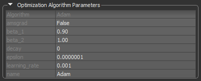
Options to set the hyperparameters of the selected optimization algorithm are available in the Optimization Algorithm Parameters box, as shown below.
Default settings for the Adam optimization algorithm
| Description | |
|---|---|
| Algorithm | Indicates the optimization algorithm selected for model training. |
| Parameters |
The parameters of the selected optimization algorithm appear here. You can find a description of each argument for the available algorithms as follows:
Adadelta… https://www.tensorflow.org/api_docs/python/tf/keras/optimizers/Adadelta#args. Adagrad… https://www.tensorflow.org/api_docs/python/tf/keras/optimizers/Adagrad#args. Adam… https://www.tensorflow.org/api_docs/python/tf/keras/optimizers/Adam#args. Adamax… https://www.tensorflow.org/api_docs/python/tf/keras/optimizers/Adamax#args. Nadam… https://www.tensorflow.org/api_docs/python/tf/keras/optimizers/Nadam#args. RMSprop… https://www.tensorflow.org/api_docs/python/tf/keras/optimizers/RMSprop#args. SGD… https://www.tensorflow.org/api_docs/python/tf/keras/optimizers/SGD#args. |
| Name |
Optional name prefix for the operations created when applying gradients. Defaults to the name of the selected optimization algorithm, for example, Adam.
Note This parameter is not available for the Adadelta and SGD optimization algorithms. |
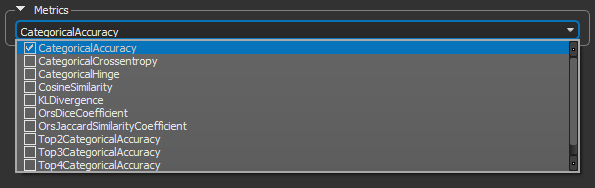
Metrics are functions that can be used to measure the performance of your model and are computed when a model is evaluated. The available metrics for estimating a model's performance are available in the Metrics drop-down menu, as shown below.
Metrics
The following metrics are available for measuring the performance of regression models.
| Description | |
|---|---|
| CosineSimilarity |
Computes the cosine similarity between the labels and predictions, in which: CosineSimilarity = (a . b) / ||a|| ||b||. References |
| LogCoshError |
Computes the logarithm of the hyperbolic cosine of the prediction error, in which: LogCoshError = log((exp(x) + exp(-x))/2), where x is the error ('y_pred' - 'y_true'). References |
| MeanAbsoluteError (MAE) |
Calculated by taking the median of all absolute differences between the target and the prediction, this metric is particularly robust to outliers.
References |
| MeanAbsolutePercentageError |
Also known as mean absolute percentage deviation (MAPD), computes the mean absolute percentage error between 'y_true' and 'y_pred'. This metric is sensitive to relative errors.
References |
| MeanSquaredError (MSE) |
Computes mean square error, which is a metric corresponding to the expected value of the squared (quadratic) error or loss.
References |
| MeanSquaredLogarithmicError |
Computes a metric corresponding to the expected value of the squared logarithmic (quadratic) error or loss.
References |
| Poisson |
Computes the Poisson metric between 'y_true' and 'y_pred', in which: Poisson= 'y_pred' - 'y_true' * log('y_pred'). References |
| PrecisionAtRecall |
Computes best precision where recall is greater than or equal to a specified value.
Note This metric creates four local variables, 'true_positives', 'true_negatives', 'false_positives', and 'false_negatives' that are used to compute the precision at the given recall. The threshold for the given recall value is computed and used to evaluate the corresponding precision. References |
| RecallAtPrecision |
Computes best recall where precision is ≥ specified value. For a given score-label-distribution the required precision might not be achievable, in this case 0.0 is returned as recall.
Note This metric creates four local variables, 'true_positives', 'true_negatives', 'false_positives', and 'false_negatives' that are used to compute the recall at the given precision. The threshold for the given precision value is computed and used to evaluate the corresponding recall. References |
| RooMeanSquaredError |
Computes root mean squared error metric between 'y_true' and 'y_pred'.
References |
The following metrics are available for measuring the performance of semantic segmentation models.
| Description | |
|---|---|
| CategoricalAccuracy |
Calculates how often predictions match 'one-hot' labels. This metric creates two local variables, 'total' and 'count' that are used to compute the frequency with which 'y_pred' matches 'y_true'. This frequency is ultimately returned as 'categorical accuracy': an idempotent operation that simply divides 'total' by 'count'.
Note 'y_pred' and 'y_true' are passed in as vectors of probabilities, rather than as labels. References |
| CategoricalCrossentropy |
Computes the crossentropy metric between the labels and predictions. Labels are given as a 'one_hot' representation. For example, when label values are [2, 0, 1], 'y_true' = [[0, 0, 1], [1, 0, 0], [0, 1, 0]].
References |
| CategoricalHinge |
Computes the categorical hinge metric between 'y_true' and 'y_pred'.
References |
| CosineSimilarity |
Computes the cosine similarity between the labels and predictions, in which: CosineSimilarity = (a . b) / ||a|| ||b||. References |
| KLDivergence |
Computes Kullback-Leibler divergence metric between 'y_true' and 'y_pred', in which: KLDivergence = 'y_true' * log('y_true' /'y_pred'). References |
| OrsDiceCoefficient | Similar to F1 score, evaluates the model's ability to maximize precision (how many positives are actually positive) and recall (how many positives were detected). |
| OrsJaccardSimilarityCoefficient | Similar to Intersection-Over-Union (IoU), evaluates the ratio of the intersection between two sets and the union of those two sets. |
| OrsTopKCategoricalAccuracy |
Computes the number of times that the correct label is among the top K (2, 3, 4, or 5) labels predicted (ranked by predicted scores).
Computes how often targets are in the top K (two, three, or four) predictions. |
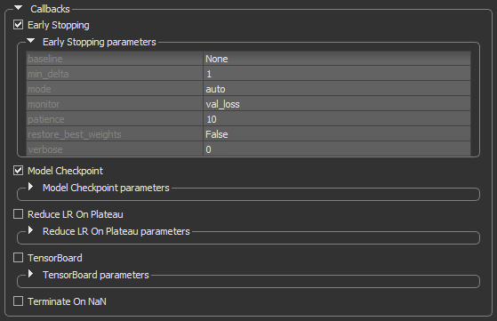
Callbacks are functions called at particular time points during the training process, usually at the end of a training epoch or at the end of batch processing. In the current version of the Deep Learning Tool, five callbacks are supported to help the training process. These are available in the Callbacks box, as shown below.
Callbacks
| Description | |
|---|---|
| Early Stopping |
Stops training upon a particular condition, for example if val_loss reaches a specific value, or if the results do not improve (see Early Stopping).
|
| Model Checkpoint | Saves the model during the training (see Model Checkpoint). |
| Reduce LR on Plateau | Reduces the learning rate (lr) when a selected metric has stopped improving (see Reduce LR on Plateau). |
| Terminate on NaN |
Terminates training when a NaN loss (Not a Number) is encountered. It is usually useful to select this callback, in order to stop training when a problem is encountered.
Note Refer to www.tensorflow.org/api_docs/python/tf/keras/callbacks/TerminateOnNaN for more information about this callback. |
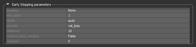
The Early Stopping callback can be set to stop training when a monitored quantity has stopped improving. This can help prevent overfitting. A good idea when using early stopping is to choose a patience level that is coherent with the selected number of epochs.
Early Stopping callback
| Description | |
|---|---|
| baseline | Is the baseline value for the monitored quantity to reach. Training will stop if the model doesn't show improvement over the baseline. |
| min_delta |
Is the minimum change in the monitored quantity to qualify as an improvement. An absolute change of less than min_delta, will count as no improvement.
|
| mode |
Determines when training will stop — Min, Max, or Auto.
Min… Training will stop when the quantity monitored has stopped decreasing. For example, when Max… Training will stop when the quantity monitored has stopped increasing. For example, when Auto… The mode — |
| monitor |
Lets you choose the quantity to be monitored, for example, val_loss.
For semantic segmentation models, the quantities that can be monitored include For regression models, the quantities that can be monitored include Note Statistics related to the monitored quantities appear on the progress bar during training and in the Training Results dialog. |
| patience | The number of epochs with no improvement after which training will be stopped. |
| restore_best_weights |
If True, the model weights from the epoch with the best value of the monitored quantity will be restored when the model is compiled. If False, the model weights obtained at the last step of training will be used.
|
| verbose | Lets you choose an option — 0 (silent) or 1 (verbose) — for producing detailed logging information. |
This callback can be configured to monitor a certain quantity during training and to save only the best model.
Model Checkpoint callback

| Description | |
|---|---|
| load_weights_on_restart | True or False (the default setting is 'False').
If |
| mode | Min, Max, or Auto (the default setting is 'Auto').
Determines if the current save file should be overwritten, based on either the minimization or maximization of the monitored quantity, and |
| monitor |
Lets you choose the quantity to be monitored, for example, val_loss.
For semantic segmentation models, the quantities that can be monitored include For regression models, the quantities that can be monitored include Note Statistics related to the monitored quantities appear on the progress bar during training and in the Training Results dialog. |
| save_best_only | True or False (the default setting is 'False')
If |
| save_freq |
Determines the frequency — epoch or an integer — in which the model is saved. The default setting is 'epoch'.
epoch… The callback saves the model after each epoch. Integer… The callback saves the model at end of a batch at which this many samples have been seen since last saving. Note that if the saving isn't aligned to epochs, the monitored metric may potentially be less reliable as it could reflect as little as 1 batch, since the metrics get reset every epoch. |
| verbose | Lets you choose an option — 0 (silent) or 1 (verbose) — for producing detailed logging information. |
This callback can automatically reduce the learning rate of the selected optimization algorithm by a specified factor when the monitored quantity stops improving. This can be especially useful when the selected optimizer does not automatically adapt its learning rate. For example, SDG (Stochastic Gradient Descent) does not adapt automatically, but Adam does.
Reduce LR on Plateau callback

| Description | |
|---|---|
| cooldown | The number of epochs to wait before resuming normal operation after the learning rate has been reduced. |
| factor | The factor by which the learning rate will be reduced. Calculated as: new_lr = lr * factor. |
| min_delta | The threshold for measuring the new optimum, to only focus on significant changes. |
| min_lr | The lower bound on the learning rate. |
| monitor |
Lets you choose the quantity to be monitored, for example, val_loss.
For semantic segmentation models, the quantities that can be monitored include For regression models, the quantities that can be monitored include |
| patience | The number of epochs with no improvement, after which learning rate will be reduced. |
| verbose | Lets you choose an option — 0 (silent) or 1 (verbose) — for producing detailed logging information. |